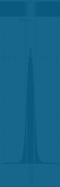
PySpectrometer3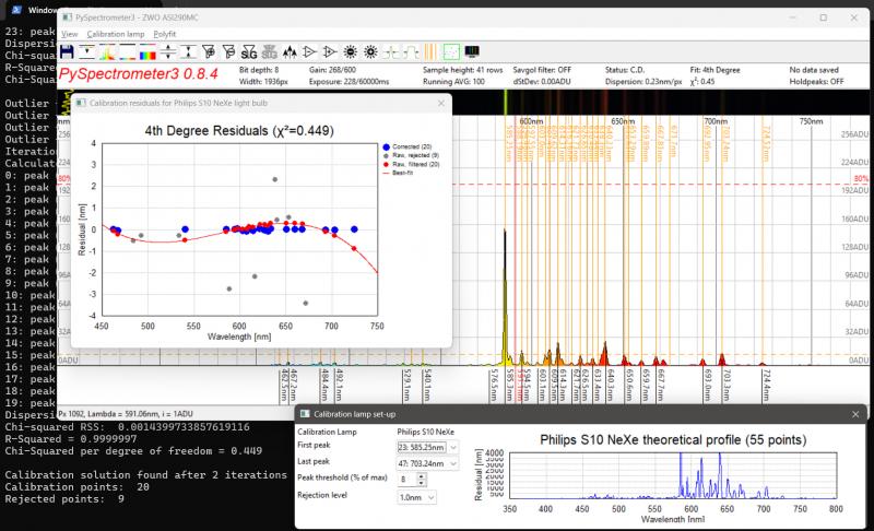 Figure 1: PySPectrometer3 with the two calibration windows opened, capturing data from an 8bit ZWO ASI290MC. At a presentation at the Dutch Astrophotography Society of the KNVWS in October 2024 Hugo Batema explained a piece of open source software he found on the internet with possible good use for astrophotographers: Les Wright's PySpectrometer2, which he developed in Python, hence the "Py" in the name. In the months following this presentation I have been working on an improved spectrometer-bench and PySpectrometer3, a Windows-based successor to PySpectrometer2 on which it still is largely based. Where the previous version was intended for use with a RaspberryPi, this new version is designed to work with Windows. Still it is developed fully open-source under Python, now using wxPython, so that any programmer can take my version to an even higher level. For the best measurements I developed an improved version of the spectrographic filter test bench. 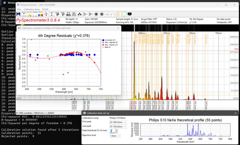 Figure 2: PySPectrometer3 with the two calibration windows opened, capturing data from a 12bit ZWO ASI290MM. Improvements Main differences with PySpectrometer2 are: - Implementation of ZWO and USB cameras (next to RaspberryPi camera) - Implementation of 12bit and 16bit mono cameras; - Variable height of sampling area; - Variable temporal running average filter; - Auto-calibration function with multiple reference spectra for commonly used lamps (Ne-Xe, Ne-Ar, and luminescence); - Selectable four orders of polyfit during calibration; - Displaying calibration lines; - Calibration quality control; - Darks; - Normalisation mode to quantify the effect of filters; - FWHM and block-wave measurement modes; - Export of 1D-fits files for further use in e.g. BASS; In order to make maximum use of above functionality it is recommended to use the software in combination with the improved spectroscope-bench shown on this site, which allows to test filters with collimated light and at various focal-ratios. 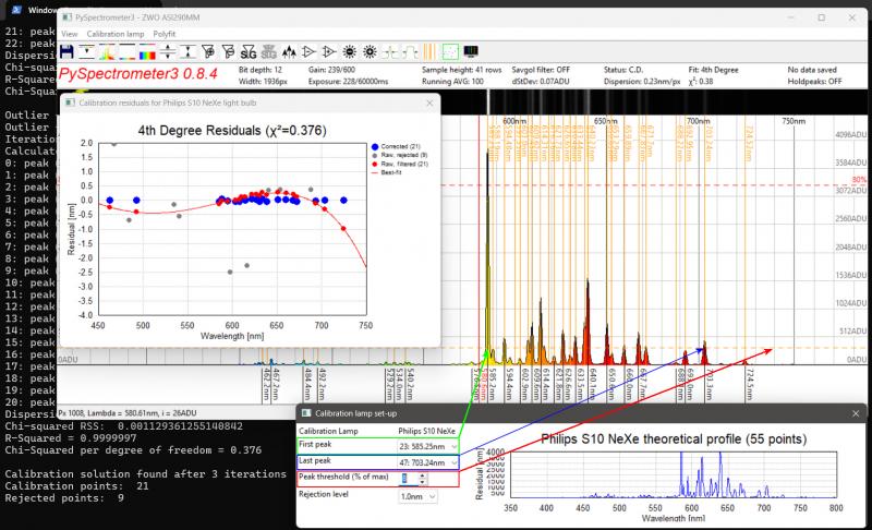 Figure 3: Setting up the calibration parameters. Calibration routine PySpectrometer3 has an almost fully automated calibration routine. In order to let it do its job, it requires a few parameters to be properly set-up (see figure 3). After having selected the correct calibration lamp in the corresponding menu, the calibration windows can be opened to set-up the calibration, either by clicking the corresponding icons in the tool-bar or pressing "=" for the spectrum window and "o" for the observation-residuals window. At first use PySpectrometer3 sets the parameters to default values that may (or not) work with your set-up. The first three parameters define how the peaks are detected in the calibration spectrum. The Peak Threshold (% of max) allows to raise and lower a dashed orange line which indicates the threshold (red rectangle in figure 3). The first and last peak that are higher than this threshold need to be set in the first two fields manually (green and blue rectangles respectively). Once set, pressing the calibrate icon in the toolbar (or "c" on the keyboard) will cause the software to calibrate the set-up using the two defined peaks as reference. For this the two peaks are taken as the truth and used to inter- and extrapolate the entire spectrum in a linear way. The Rejection Level can be used to reject any peaks that are found at a distance of more that the set wavelengths from the value found with this linear fit. Once this first step is done, PySpectrometer3 tries to fit the found peaks using the polyfit setting in the corresponding menu (usually a 3rd or 4th order would produce good results) and displays the residuals in the observations plot window. Based on the dispersion and residuals of the best-fit the Chi-Squared per Degree of Freedom (χ2) is calculated. A good solution should have a χ2 of around 1. A very low χ2 means that the order of the polynome is too high, a very high χ2 means that (some of) the spectral lines are not well formed due to overexposure, that the wrong lamp has been chosen, or that the calibration lamp deviated from what is known in the software. It is recommended not to over-expose the camera too much during calibration as that will affect the shape of the top-part of the peaks in the spectrum, making them square, and resulting in a poor calibration. Flats and darksIn addition to the normalisation (you could call this a flat, press "n" to activate) I also built in the possibility to take darks (press "-"). At the moment this is still done at the output level: the images from the camera are first processed and shown as a graph, after which this graph can serve as a dark. The advantage of this method is that the dark is one-dimensional, which makes processing it fast and the dark can also be easily saved in the ini-file. Filtering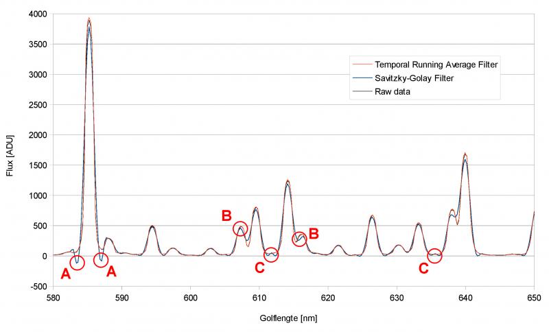 Figure 4: Artifacts (A), shifted maxima (B) and non-existent lines (C) due to the Savitzky-Golay filter. Next up was filtering. PySpectrometer2 uses a Savitzky-Golay (SG) filter for this. The SG filter is a smoothing filter that works in the direction of the horizontal axis of the graph. It is an improved variant of the running average filter, but then by means of convolution, in which a polynomial is fitted to the data by means of a linear least squares method (the order of the polynomial is adjustable). Now there are various ways to smooth spectrometer data, but a running average and SG filter are not the best options, since these filters cannot handle the sudden intensity transitions of the spectral lines. This creates unwanted artefacts (see figure 4, A), shifted spectral lines (B) and even new spectral lines (C). It is therefore better to use column stacking and live stacking (the SG filter is still built in, but is disabled by default). Column stacking is already built into PySpectrometer2, albeit rudimentary over only 3 rows of pixels. Since the spectral lines illuminate approximately 170 rows of pixels of the imaging chip, it is possible to calculate averages over a larger range. In PySpectrometer2 these are 3 rows, in PySpectrometer3 this has been expanded to an adjustable number of rows of pixels from 1 to 41, from which the average is determined (since the spectral lines are slightly curved, the 41 pixels are a safe margin within which they are still somewhat straight). It is important to align the camera and spectroscope well with each other, so that the spectral lines actually run parallel to the columns of the imaging chip, this in order to prevent smearing. Incidentally, the spectrum and the spectral lines shown within it are not completely perpendicular to each other, so the importance is to align the lines neatly, the spectrum as a whole may be tilted. 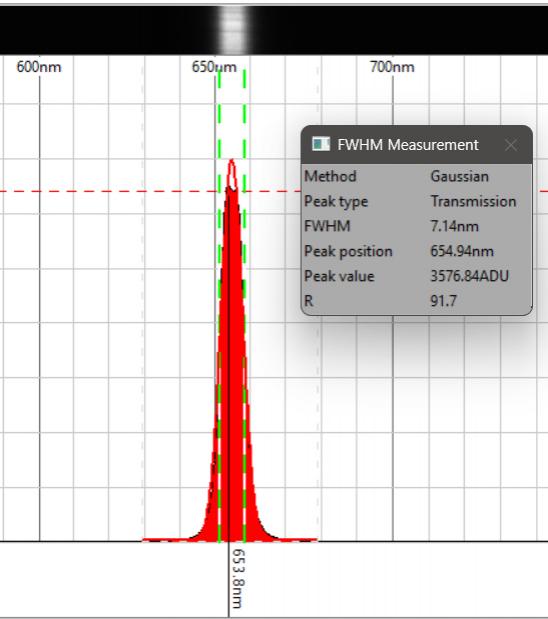 Figure 5: FWHM measurement of a 7nm bandpass H-alpha filter. Live stacking was not yet present in PySpectrometer2. In PySpectrometer3 this is set to 30 frames by default and can be set as desired with 1 frame as a lower limit (there is no upper limit). This filter works as a temporal running average: instead of smoothing the graph by looking at the adjacent pixels, the smoothing takes place in time, so over a number of recordings. This does have the disadvantage that the software needs time to show a stable graph. By now subtracting each new graph shown from the previous one and calculating and showing the standard deviation of the difference (as dStDev), the user is informed about the stability of the result. The reset button (press "x") allows to reset the temporal running average, by which it starts with the last captured image. To make the software really useful, two measurement methods have been built in to measure the full width half maximum (FWHM) of a spectral line or a filter response. One method works on the basis of a Gaussian curve fit, the second on the basis of a block fit. The first method attempts to fit a Gaussian curve through the data. This works well if the data actually has a Gaussian shape, but is less or even unsuitable if the data has a block shape, such as with a luminance filter. In the latter case, the edges of the block shape are determined and the FWHM is calculated from them. Both methods work for both transmission and absorption spectra. In figure 5 the FWHM measurement of an H-alpha filter is shown. The unfitted peak value is found at 653.8nm (the top of the peak is flattened), the Gaussian best fit at 654.94nm (H-alpha is at 656.28nm). The FWHM is found to be 7.14nm, corresponding to the 7nm stated by ZWO. Quality indicatorsIt is great that we can now actually start measuring, but of course we want to know how accurate the software works. Above we saw the introduction of the dStDev which indicates how stable the measurement is, and in addition it also indicates what the dispersion is (the amount of wavelength per pixel). Of course we also want to know how well the calibration of the system has been performed. Calibration is done with the previously mentioned calibration lamps, whereby the found spectral lines are fitted as well as possible in their theoretical values. PySpectrometer2 only gave the R-squared (R2) in the terminal. The closer this value is to 1, the better the fit. What PySpectrometer2 did not show is the reason why R2 deviates from 1. It may well be that one or more spectral lines do not fit well, but that this does not significantly affect the fit. In PySpectrometer3 the calibration process is largely automated (see figure 3). After opening the Calibration lamp set-up screen a horizontal dotted line appears in the graph which can be adjusted in height. The user now only has to indicate which are the first and last spectral lines that intersect this dotted line in intensity, the calibration routine will now determine all other spectral lines (both between the two and outside them) and make a best-fit with them (this can be linear up to and including a fourth-order polynomial), and calculate the R2 and the chi-squared per degree of freedom (χ2). The latter should also be close to 1 as an indication of a good best-fit (a value much smaller than 1 indicates that the order of the polynomial is too large). If the Calibration Residuals screen is also opened, it can also be seen which spectral lines are not well resolved and what the shape of the polynomial is. Supported calibration lampsPySpectrometer3 can now handle four different calibration lamps: the fluorescent lamp from PySpectrometer2, and the Philips S10, Shelyak S0148 and Relco-SC480 gas discharge lamps mentioned in the Filter test-bench page. The software has been extensively tested with the first three and example graphs are available in the Calibration lamp setup screen. The theoretical wavelengths are taken from the work of Walker and Thompson and supplemented with data from Typical Spectra of Oriel Instruments Spectral Calibration Lamps.1 Example measurements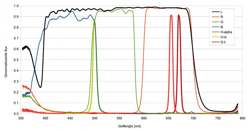 Figure 6: ZWO unmounted 36mm LRGB and narrowband filter set. With PySpectrometer3 it is now possible to perform qualitative measurements on filters (of course within the limitations of the spectroscope and calibration lamp used). In figure 6 the measurement of a ZWO 36mm unmounted filter set for LRGB and narrowband is shown. It can be clearly seen that on the red side of the spectrum the luminance and red filters almost coincide and that the O-iii filter coincides with the overlapping area of blue and green. On the blue side of the spectrum it can be seen that the luminance filter is not dense and at 360nm even still lets through approximately 60% of the photons. Green and red also let through 17% and 26% of the light respectively. It can also be seen that the transmission increases slightly with increasing wavelength. The graph was made in a spreadsheet program using exported .csv data from PySpectrometer3. 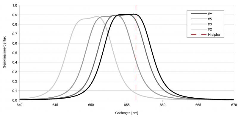 Figure 7: Bandpass shift due to f-number on a ZWO 7nm H-alpha filter. In figure 7 the effect of the f-number on the bandpass of a ZWO 7nm bandpass H-alpha filter is shown. The red vertical line is the wavelength of H-alpha that we are trying to capture, the curves show the measured bandpass of the filter at varying incidence of the broadband light of the setup. It is clearly visible that, as the angle of incidence of the light deviates further from the normal (decreasing f-number), the range of the filter shifts towards the blue side of the spectrum. At f/10 (not in the graph) the difference with perpendicular incidence of the light (f/∞) is so small that there was no point in showing that line. At f/5 the signal loss is only 7%, at f/3 already 49% and at f/2 no less than 83%! In addition, the transmission decreases and the bandpass becomes slightly narrower (in this case from approximately 7.2nm to approximately 6.7nm). All in all this means that when we take pictures with a very fast telescope, it is as if we are stopping down the lens.2 With filters with an even smaller bandpass of 3nm for example, this effect will be more prominent and it will therefore appear as if the telescope has been stopped down even more. With very fast systems with a central obstruction, such as a Celestron RASA, in combination with a very small bandpass of 2nm, no light will even reach the sensor at all, because the resulting aperture becomes smaller than the central obstruction.2 Change log0.8.6 (17/11/2025): Ensured normalisation is done with floats, solving apparent 'light-leakage' near the low-intensity ends of the spectrum. 0.8.5 (23/06/2025): Added Temporal Running Average Reset-button, Temporal Running Average Counter, and Stability-indicator 0.8.4 (10/06/2025): First stable version Notes[1]: See the Filter test-bench page for details.[2]: Thompson, J., 'Narrowband Filters & Fast Optics (A match made in heaven, or is it?)', in: Astronomy Technology Today vol.15, iss.2, (2021), p.62. If you have any questions and/or remarks please let me know. |
InFINNity Deck... Astrophotography... Astro-Software... Astro Reach-out... Equipment... White papers...
ASCOM Envir. SafetyMonitor ASCOM File SafetyMonitor ASCOM Generic UPS driver ASCOM IP SafetyMonitor ASCOM SafetyMonitor Hub Astronomical Twilight FITSalize Log10mGrabber MountCMD MountMonitor PySpectrometer3